Using LOOKUP
- Excel Basics
- Adding Information
- Clipart
- Formulas with Autosum
- Advanced Formulas
- AutoFill
- Using LOOKUP (text)
- Using LOOKUP (video)
- Creating Charts
LOOKUP is a very useful Excel function to understand. LOOKUP's essential use is to translate numerical data into categories of non-numerical data that you specify. For instance, translating percentages to grade letters in a gradebook is an ideal use of LOOKUP. Another use for LOOKUP might be to translate temperatures in degrees to categories, such as moderate, cold, warm, and so forth.
To use LOOKUP within an Excel spreadsheet, follow these steps:
1. First, enter your numerical data into your spreadsheet. For example, if you were creating a gradebook you might have all of your students' grades listed in a column form. In this example, we will use the Percentage data.
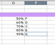
2. You must next set up your LOOKUP criteria range (known as an array) by entering the desired correlations of numerical data and non-numerical category names elsewhere in your spreadsheet. So, in our example of the gradebook, values between 50% and 59% equal an F, values between 60% and 69% equal a D, and so on. This information must be entered into the spreadsheet, which creates your array. Note that LOOKUP arrays must be entered starting with the lowest criteria value and ending with the highest, as shown below.
3. Note the row-column location of your array and return to the body of your spreadsheet. In the column or row where you would like LOOKUP data to appear, begin a new formula in the first cell by typing =.
Next, type the following information into the cell, putting your data in place of the italicized entries:
=LOOKUP(cell name of data to be compared to the array, cell at the top left corner of your array:cell at the lower right corner of your array)
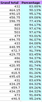
So, in our example, we are starting our LOOKUP comparison with Cell L4, which contains the first percentage in our gradebook. Our array runs from O4 to P9. To prepare ourselves for AutoFill, the $'s have been added before the O, 4, P, and 9 to keep the reference absolute (please see the section on AutoFill for more information).
Your completed formula should look something like this:
![]()
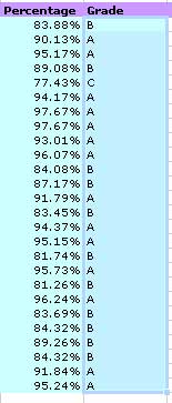
4. Press Return and the formula should show the correct entry from your array. This student's grade was between 80% and 89%, so the correct grade letter is shown as a B.
![]()
5. If this were a gradebook, you would have many students to work with. If you used an absolute reference in your formula as shown above, you can drag the AutoFill handle down through your entire gradebook to recalculate the formula for each student. While it is not necessary to use absolute references in any formula, using them does enhance your ability to use AutoFill, which can save you a great deal of time. Please see the section on AutoFill for additional information.