Creating Charts
- Excel Basics
- Adding Information
- Clipart
- Formulas with Autosum
- Advanced Formulas
- AutoFill
- Using LOOKUP (text)
- Using LOOKUP (video)
- Creating Charts
Charts and graphs may be created in Excel using a tool known as the Chart Wizard. The Chart Wizard can lead you through all the steps necessary to add a variety of different charts and graphs to your spreadsheet.
When you create a chart, keep in mind that it should illustrate your data in a manner that makes the most sense. So, for example, a pie chart would be useful for illustrating the demographics in the population of a country, but it would not be appropriate for comparing the scores of two individuals taking the SAT. For this latter situation, a column or bar graph would be a more logical representation.
To create a chart or graph:
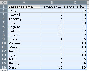
1. Highlight the data in your spreadsheet that you wish to illustrate, including any appropriate text labels such as student names, product types, demographic types, etc.
NOTE: You do not have to do this step first, as the opportunity to select your chart information will appear later, but some users prefer to select chart data first, rather than later.
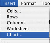
2. Click the Chart Wizard icon from the Standard toolbar, OR click the Insert menu and choose Chart.
![]()
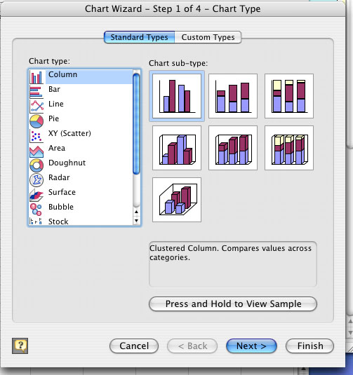
3. A list of chart types will appear. Choose the chart type and style that is most appropriate for your particular application, then click Next.
4. If you did not already, choose the data range in your spreadsheet that will be charted. You will be able to see a preview of your chart -- if it does not appear as it should, change the data range as necessary. Click Next to continue.
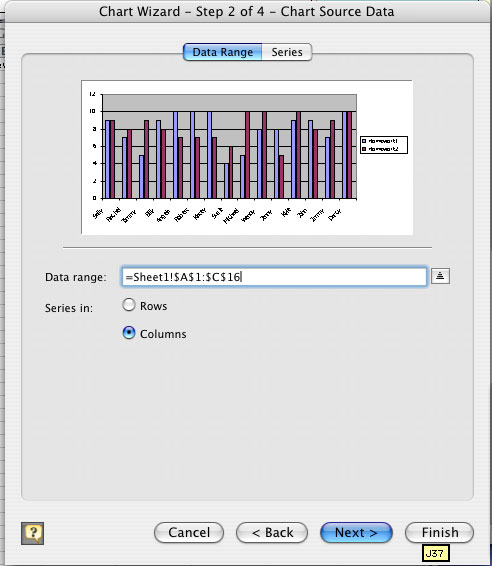
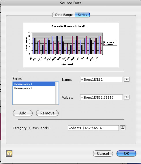
In the Series Tab of this step, you may also change the labels that appear in the chart legend and individual data sources of each data series. This is an option for further customizing your chart, but it is not a necessity for completion.
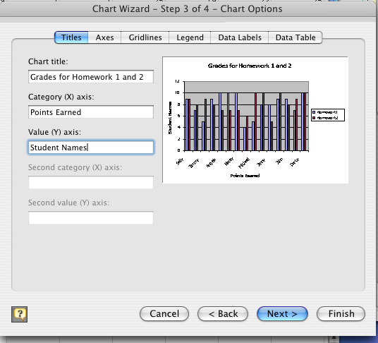
5. Step 3 allows you to add titles and customize the appearance of your chart by adding gridlines, changing the location and size of the legend, and adding labels and additional tables to your chart. All of these items are options that you may or may not wish to use depending on your situation. When you are ready, click Next to continue.
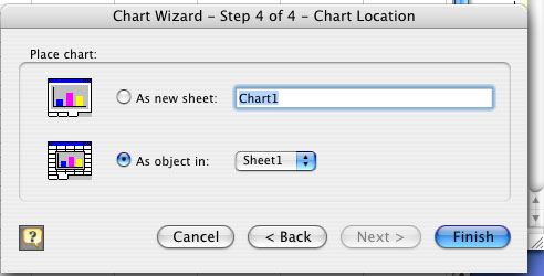
6. The final step of the Chart Wizard is choosing the location for your chart. You may decide to embed it into an existing worksheet, or to create a new worksheet that shows only the graph (for more information on worksheets, see Microsoft Excel Basics).